2장 수출의 내용을 따져보자#
출처: UNCTAD (2012), A Practical Guide to Trade Policy Analysis, Chapter 1.
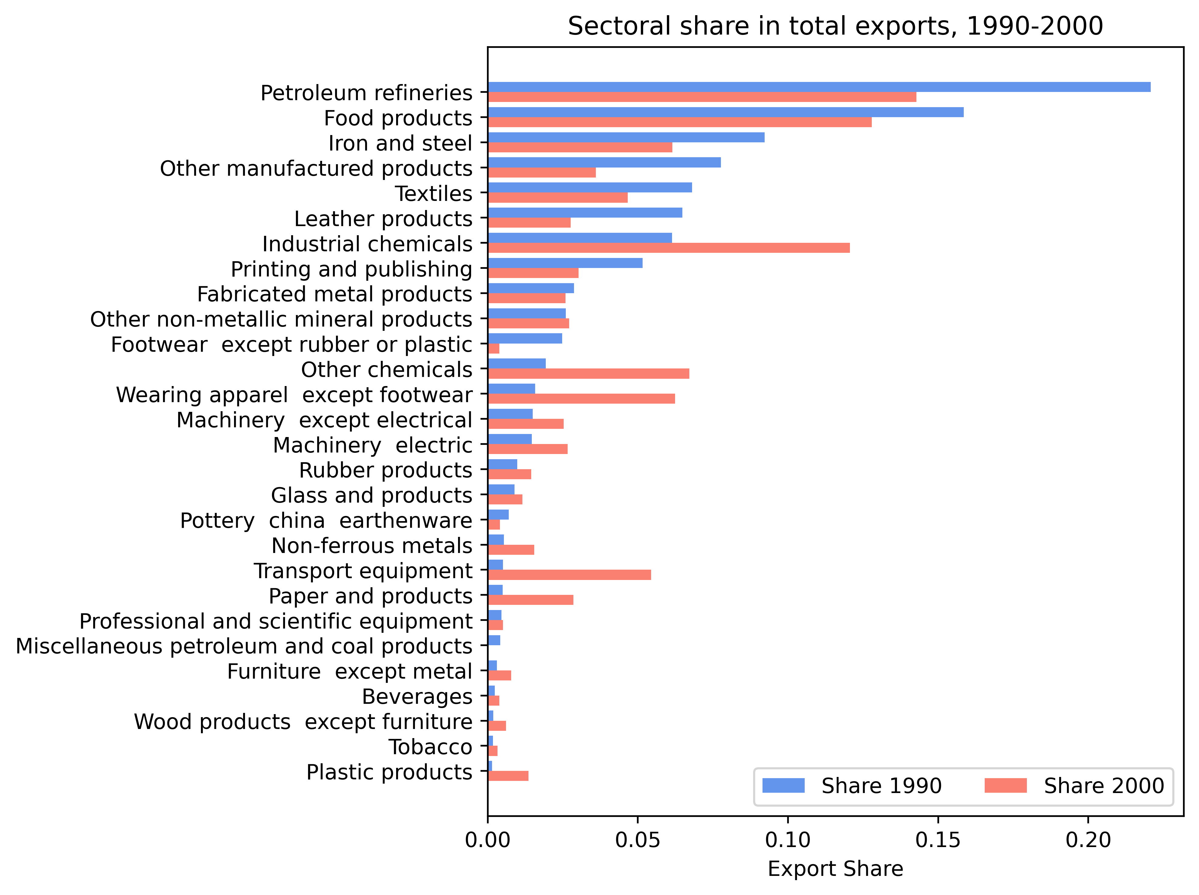
1. 수출의 부문별 비중#
한 국가의 수출이 어느 부문(sector)에 집중되어 있는지를 분석한다.
아래 예는 콜롬비아를 대상으로 1990년과 2000년 전체 수출액에서 각 생산 부문(ISIC 3자리)이 차지하는 비중을 계산해서 막대그래프로 제시한다.(ISIC는 UN의 국제표준산업분류다.)
석유정제(petroleum refineries) 산업이 1990년과 2000년 모두 주요 수출 부문을 구성했지만, 1990년에는 전체 수출의 20% 이상을 차지하던 비중이 2000년에는 15% 미만으로 감소했다.
반면에 산업용화학제품(industrial chemicals), 화학제품(other chemicals), 의류(wearing apparel except footwear), 운송장비(transport equipment)의 비중은 같은 기간 동안 모두 증가했다. 예를 들어, 운송장비의 전체 수출 비중은 1% 미만에서 5% 이상으로 성장했다.
데이터#
import pandas as pd
import numpy as np
import matplotlib.pyplot as plt

# TPP.dta 파일 읽기
df = pd.read_stata("../Data/TPP.dta")
df
| sector | ccode | year | isic3d_3dig | wage_bill | value_added | output | n_female_emp | n_establ | n_employees | ... | tar_sdahs | tar_minahs | tar_maxahs | tar_savg_mfn | tar_iwmfn | tar_sdmfn | tar_minmfn | tar_maxmfn | tar_hs_lines | id | |
|---|---|---|---|---|---|---|---|---|---|---|---|---|---|---|---|---|---|---|---|---|---|
| 0 | Food products | ARG | 1976 | 311 | NaN | NaN | NaN | NaN | NaN | 302783.0 | ... | NaN | NaN | NaN | NaN | NaN | NaN | NaN | NaN | NaN | 1.0 |
| 1 | Food products | ARG | 1977 | 311 | NaN | NaN | NaN | NaN | NaN | 289400.0 | ... | NaN | NaN | NaN | NaN | NaN | NaN | NaN | NaN | NaN | 1.0 |
| 2 | Food products | ARG | 1978 | 311 | NaN | NaN | NaN | NaN | NaN | 258174.0 | ... | NaN | NaN | NaN | NaN | NaN | NaN | NaN | NaN | NaN | 1.0 |
| 3 | Food products | ARG | 1979 | 311 | NaN | NaN | NaN | NaN | NaN | 257338.0 | ... | NaN | NaN | NaN | NaN | NaN | NaN | NaN | NaN | NaN | 1.0 |
| 4 | Food products | ARG | 1980 | 311 | NaN | NaN | NaN | NaN | NaN | 244513.0 | ... | NaN | NaN | NaN | NaN | NaN | NaN | NaN | NaN | NaN | 1.0 |
| ... | ... | ... | ... | ... | ... | ... | ... | ... | ... | ... | ... | ... | ... | ... | ... | ... | ... | ... | ... | ... | ... |
| 81195 | Other manufactured products | ZAF | 2000 | 390 | 102427.867188 | NaN | NaN | NaN | NaN | 22030.0 | ... | NaN | NaN | NaN | NaN | NaN | NaN | NaN | NaN | NaN | 2800.0 |
| 81196 | Other manufactured products | ZAF | 2001 | 390 | 90033.312500 | NaN | NaN | NaN | NaN | 18168.0 | ... | 9.13 | 0.0 | 30.0 | 6.44 | 3.13 | 9.33 | 0.0 | 30.0 | 187.0 | 2800.0 |
| 81197 | Other manufactured products | ZAF | 2002 | 390 | 82382.859375 | NaN | NaN | NaN | NaN | 18571.0 | ... | NaN | NaN | NaN | NaN | NaN | NaN | NaN | NaN | NaN | 2800.0 |
| 81198 | Other manufactured products | ZAF | 2003 | 390 | NaN | NaN | NaN | NaN | NaN | NaN | ... | NaN | NaN | NaN | NaN | NaN | NaN | NaN | NaN | NaN | 2800.0 |
| 81199 | Other manufactured products | ZAF | 2004 | 390 | NaN | NaN | NaN | NaN | NaN | NaN | ... | 9.14 | 0.0 | 30.0 | 6.23 | 1.88 | 9.22 | 0.0 | 30.0 | 187.0 | 2800.0 |
81200 rows × 40 columns
변수 설명
ccode: 국가 식별 코드year: 연도exp_tv: 총수출액sector: 부문 코드(ISIC 3자리)
수출의 부문별 비중 계산#
# 각 나라, 연도별 총수출액 계산 (by ccode & year)
df['total_export'] = df.groupby(['ccode', 'year'])['exp_tv'].transform('sum')

# 각 행의 수출 비중 계산
df['export_share'] = df['exp_tv'] / df['total_export']

# 각 국가, 연도별로 export_share를 내림차순 정렬
df = df.sort_values(by=['ccode', 'year', 'export_share'], ascending=[True, True, False])

# 각 나라, 연도별 순위 생성
df['ranking'] = df.groupby(['ccode', 'year']).cumcount() + 1

# 필요한 변수만 선택
df = df[['ranking', 'sector', 'ccode', 'year', 'export_share']]

# 국가 코드와 부문(sector)별 그룹 id 생성
df['id'] = df.groupby(['ccode', 'sector']).ngroup()

# 'year'에 따라 데이터를 wide 형식으로 변환
df_wide = df.pivot(index=['id', 'ccode', 'sector'],
                   columns='year', values=['ranking', 'export_share'])
df_wide.columns = [f"{var}{year}" for var, year in df_wide.columns]
df_wide = df_wide.reset_index()

# 데이터 확인
df_wide.head()
| id | ccode | sector | ranking1976 | ranking1977 | ranking1978 | ranking1979 | ranking1980 | ranking1981 | ranking1982 | ... | export_share1995 | export_share1996 | export_share1997 | export_share1998 | export_share1999 | export_share2000 | export_share2001 | export_share2002 | export_share2003 | export_share2004 | |
|---|---|---|---|---|---|---|---|---|---|---|---|---|---|---|---|---|---|---|---|---|---|
| 0 | 0 | ARG | Beverages | 2.0 | 2.0 | 2.0 | 2.0 | 15.0 | 18.0 | 17.0 | ... | 0.012418 | 0.011486 | 0.012894 | 0.014669 | 0.014807 | 0.015941 | 0.014962 | 0.013227 | 0.013902 | 0.014117 |
| 1 | 1 | ARG | Fabricated metal products | 23.0 | 23.0 | 23.0 | 23.0 | 14.0 | 13.0 | 11.0 | ... | 0.011464 | 0.010508 | 0.010598 | 0.009396 | 0.009107 | 0.008476 | 0.009707 | 0.008798 | 0.007129 | 0.008367 |
| 2 | 2 | ARG | Food products | 1.0 | 1.0 | 1.0 | 1.0 | 1.0 | 1.0 | 1.0 | ... | 0.409555 | 0.444625 | 0.405617 | 0.400990 | 0.418084 | 0.361353 | 0.344330 | 0.387948 | 0.429200 | 0.428940 |
| 3 | 3 | ARG | Footwear except rubber or plastic | 7.0 | 7.0 | 7.0 | 7.0 | 23.0 | 23.0 | 21.0 | ... | 0.004714 | 0.003190 | 0.004530 | 0.002652 | 0.001026 | 0.000458 | 0.000257 | 0.000382 | 0.000593 | 0.000629 |
| 4 | 4 | ARG | Furniture except metal | 9.0 | 9.0 | 9.0 | 9.0 | 27.0 | 28.0 | 27.0 | ... | 0.003738 | 0.005327 | 0.005318 | 0.005233 | 0.008005 | 0.011327 | 0.012977 | 0.012310 | 0.009833 | 0.007449 |
5 rows × 61 columns
# 필요 변수 선택
cols_order = ['sector', 'ccode', 'ranking1990', 'ranking2000', 'export_share1990', 'export_share2000']
df_wide = df_wide[cols_order]

# Colombia 데이터만 선택
df_wide = df_wide[df_wide['ccode'] == "COL"]

# 정렬: ranking1990 기준 내림차순
df_wide = df_wide.sort_values(by='ranking1990', ascending=False)

# 데이터 확인
df_wide
| sector | ccode | ranking1990 | ranking2000 | export_share1990 | export_share2000 | |
|---|---|---|---|---|---|---|
| 522 | Plastic products | COL | 28.0 | 19.0 | 0.001494 | 0.013567 |
| 528 | Tobacco | COL | 27.0 | 27.0 | 0.001751 | 0.003245 |
| 531 | Wood products except furniture | COL | 26.0 | 22.0 | 0.001892 | 0.006064 |
| 504 | Beverages | COL | 25.0 | 26.0 | 0.002344 | 0.003866 |
| 508 | Furniture except metal | COL | 24.0 | 21.0 | 0.003057 | 0.007803 |
| 515 | Miscellaneous petroleum and coal products | COL | 23.0 | 28.0 | 0.004177 | 0.000092 |
| 525 | Professional and scientific equipment | COL | 22.0 | 23.0 | 0.004604 | 0.005125 |
| 520 | Paper and products | COL | 21.0 | 11.0 | 0.005006 | 0.028522 |
| 529 | Transport equipment | COL | 20.0 | 7.0 | 0.005112 | 0.054375 |
| 516 | Non-ferrous metals | COL | 19.0 | 17.0 | 0.005408 | 0.015517 |
| 523 | Pottery china earthenware | COL | 18.0 | 24.0 | 0.007001 | 0.004101 |
| 509 | Glass and products | COL | 17.0 | 20.0 | 0.008919 | 0.011551 |
| 526 | Rubber products | COL | 16.0 | 18.0 | 0.009845 | 0.014471 |
| 513 | Machinery electric | COL | 15.0 | 14.0 | 0.014725 | 0.026641 |
| 514 | Machinery except electrical | COL | 14.0 | 16.0 | 0.014967 | 0.025309 |
| 530 | Wearing apparel except footwear | COL | 13.0 | 5.0 | 0.015791 | 0.062391 |
| 517 | Other chemicals | COL | 12.0 | 4.0 | 0.019299 | 0.067106 |
| 507 | Footwear except rubber or plastic | COL | 11.0 | 25.0 | 0.024783 | 0.003902 |
| 519 | Other non-metallic mineral products | COL | 10.0 | 13.0 | 0.026064 | 0.027148 |
| 505 | Fabricated metal products | COL | 9.0 | 15.0 | 0.028717 | 0.025915 |
| 524 | Printing and publishing | COL | 8.0 | 10.0 | 0.051598 | 0.030241 |
| 510 | Industrial chemicals | COL | 7.0 | 3.0 | 0.061387 | 0.120663 |
| 512 | Leather products | COL | 6.0 | 12.0 | 0.064817 | 0.027586 |
| 527 | Textiles | COL | 5.0 | 8.0 | 0.068067 | 0.046617 |
| 518 | Other manufactured products | COL | 4.0 | 9.0 | 0.077638 | 0.036042 |
| 511 | Iron and steel | COL | 3.0 | 6.0 | 0.092231 | 0.061497 |
| 506 | Food products | COL | 2.0 | 2.0 | 0.158549 | 0.127913 |
| 521 | Petroleum refineries | COL | 1.0 | 1.0 | 0.220759 | 0.142733 |
# 부문명을 y축 레이블로 사용 (정렬된 순서 유지)
y_pos = np.arange(len(df_wide))
bar_height = 0.4

plt.figure(figsize=(8, 6), dpi=500)
plt.barh(y_pos + bar_height/2, df_wide['export_share1990'],
         height=bar_height, color='cornflowerblue', label="Share 1990")
plt.barh(y_pos - bar_height/2, df_wide['export_share2000'],
         height=bar_height, color='salmon', label="Share 2000")
plt.yticks(y_pos, df_wide['sector'])
plt.xlabel("Export Share")
plt.title("Sectoral share in total exports, 1990-2000")
plt.legend(ncol=2)
plt.tight_layout()
plt.show()
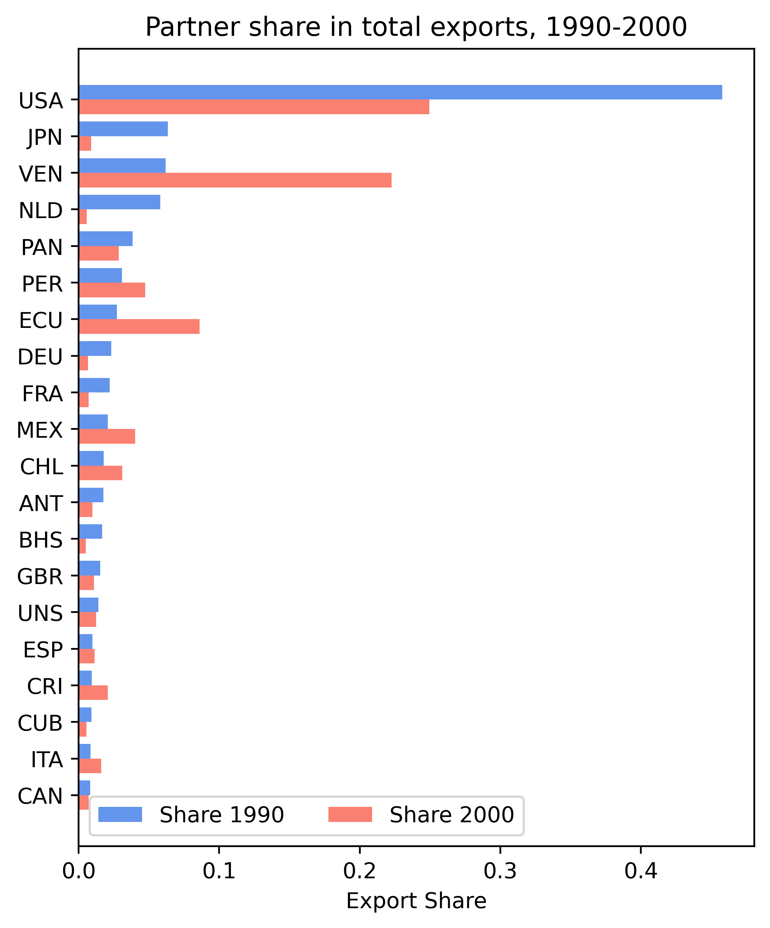
2. 수출의 나라별 비중#
한 국가의 수출이 어느 나라에 집중되어 있는지를 분석한다.
아래 예는 콜롬비아를 대상으로 1990년과 2000년 전체 수출액에서 대상국 각 나라가 차지하는 비중을 계산해서 막대그래프로 제시한다.
미국이 1990년과 2000년 모두 가장 중요한 수출 대상국임을 보여주지만, 미국으로의 수출 비중이 1990년에는 45% 이상이었으나 2000년에는 약 25%로 감소했다.
반면, 베네수엘라, 에콰도르, 페루와 같은 인접 국가로의 수출 비중은 이 기간 동안 증가한 것을 확인할 수 있다.
데이터#
import pandas as pd
import numpy as np
import matplotlib.pyplot as plt

# aBilateralTrade.dta 파일 읽기
df = pd.read_stata("../Data/aBilateralTrade.dta")
df
| ccode | pcode | year | exp_tv | imp_tv | |
|---|---|---|---|---|---|
| 0 | ABW | AIA | 2002 | 773.573975 | 0.000000 |
| 1 | ABW | AIA | 2003 | 63.463001 | 0.000000 |
| 2 | ABW | ALB | 2004 | 0.000000 | 9.815000 |
| 3 | ABW | ANT | 1995 | 475.063997 | 1518.088998 |
| 4 | ABW | ANT | 1996 | 350.091993 | 1608.835018 |
| ... | ... | ... | ... | ... | ... |
| 403130 | ZWE | ZMB | 1999 | 54505.525404 | 16210.871972 |
| 403131 | ZWE | ZMB | 2000 | 69688.172039 | 0.000000 |
| 403132 | ZWE | ZMB | 2001 | 9792.663770 | 12135.245145 |
| 403133 | ZWE | ZMB | 2002 | 175256.748111 | 17891.870960 |
| 403134 | ZWE | ZMB | 2004 | 59845.737700 | 18475.593896 |
403135 rows × 5 columns
변수 설명
ccode: 기준국 코드pcode: 상대국 코드year: 연도exp_tv: 총수출액imp_tv: 총수입액
수출의 나라별 비중 계산#
# 각 나라, 연도별 총수출액 계산 (by ccode & year)
df['tot_exp'] = df.groupby(['ccode', 'year'])['exp_tv'].transform('sum')

# 각 행의 수출 비중 계산
df['export_share'] = df['exp_tv'] / df['tot_exp']

# 내림차순 정렬 (ccode, year별로 export_share 기준)
df = df.sort_values(by=['ccode', 'year', 'export_share'], ascending=[True, True, False])

# 그룹별 순위 생성
df['ranking'] = df.groupby(['ccode', 'year']).cumcount() + 1

# 필요한 변수 선택
df = df[['ranking', 'ccode', 'pcode', 'year', 'export_share']]

# 국가 코드와 파트너 코드별 그룹 id 생성
df['id'] = df.groupby(['ccode', 'pcode']).ngroup()

# 'year'에 따라 데이터를 wide 형식으로 변환
df_wide = df.pivot(index=['id', 'ccode', 'pcode'],
                   columns='year', values=['ranking', 'export_share'])
df_wide.columns = [f"{var}{year}" for var, year in df_wide.columns]
df_wide = df_wide.reset_index()

# 데이터 확인
df_wide.head()
| id | ccode | pcode | ranking1976 | ranking1977 | ranking1978 | ranking1979 | ranking1980 | ranking1981 | ranking1982 | ... | export_share1995 | export_share1996 | export_share1997 | export_share1998 | export_share1999 | export_share2000 | export_share2001 | export_share2002 | export_share2003 | export_share2004 | |
|---|---|---|---|---|---|---|---|---|---|---|---|---|---|---|---|---|---|---|---|---|---|
| 0 | 0 | ABW | AIA | NaN | NaN | NaN | NaN | NaN | NaN | NaN | ... | NaN | NaN | NaN | NaN | NaN | NaN | NaN | 0.006742 | 0.000919 | NaN |
| 1 | 1 | ABW | ALB | NaN | NaN | NaN | NaN | NaN | NaN | NaN | ... | NaN | NaN | NaN | NaN | NaN | NaN | NaN | NaN | NaN | 0.0 |
| 2 | 2 | ABW | ANT | NaN | NaN | NaN | NaN | NaN | NaN | NaN | ... | 0.161659 | 0.141906 | 0.129129 | 0.063667 | NaN | NaN | NaN | NaN | NaN | NaN |
| 3 | 3 | ABW | ARE | NaN | NaN | NaN | NaN | NaN | NaN | NaN | ... | NaN | NaN | NaN | NaN | NaN | 0.000006 | 0.0 | NaN | 0.001144 | 0.0 |
| 4 | 4 | ABW | ARG | NaN | NaN | NaN | NaN | NaN | NaN | NaN | ... | 0.000871 | 0.000000 | NaN | 0.000000 | NaN | 0.000270 | 0.0 | 0.000334 | 0.001108 | 0.0 |
5 rows × 61 columns
# 필요 변수 선택
cols_order = ['ccode', 'pcode', 'ranking1990', 'ranking2000',
              'export_share1990', 'export_share2000']
df_wide = df_wide[cols_order]

# Colombia 데이터만 선택
df_wide = df_wide[df_wide['ccode'] == "COL"]

# 정렬: ranking1990 기준 내림차순
df_wide = df_wide.sort_values(by='ranking1990', ascending=False)

# 상위 20개 파트너만 선택
df_wide = df_wide[df_wide['ranking1990'] <= 20]

# 데이터 확인
df_wide.head()
| ccode | pcode | ranking1990 | ranking2000 | export_share1990 | export_share2000 | |
|---|---|---|---|---|---|---|
| 6359 | COL | CAN | 20.0 | 23.0 | 0.008298 | 0.007027 |
| 6427 | COL | ITA | 19.0 | 11.0 | 0.008500 | 0.016025 |
| 6372 | COL | CUB | 18.0 | 28.0 | 0.009235 | 0.005582 |
| 6370 | COL | CRI | 17.0 | 9.0 | 0.009349 | 0.020759 |
| 6388 | COL | ESP | 16.0 | 13.0 | 0.009744 | 0.011477 |
y_pos = np.arange(len(df_wide))
plt.figure(figsize=(5, 6), dpi=500)

plt.barh(y_pos + bar_height/2, df_wide['export_share1990'],
         height=bar_height, color='cornflowerblue', label="Share 1990")
plt.barh(y_pos - bar_height/2, df_wide['export_share2000'],
         height=bar_height, color='salmon', label="Share 2000")
plt.yticks(y_pos, df_wide['pcode'])
plt.xlabel("Export Share")
plt.title("Partner share in total exports, 1990-2000")
plt.legend(ncol=2)
plt.tight_layout()
plt.show()
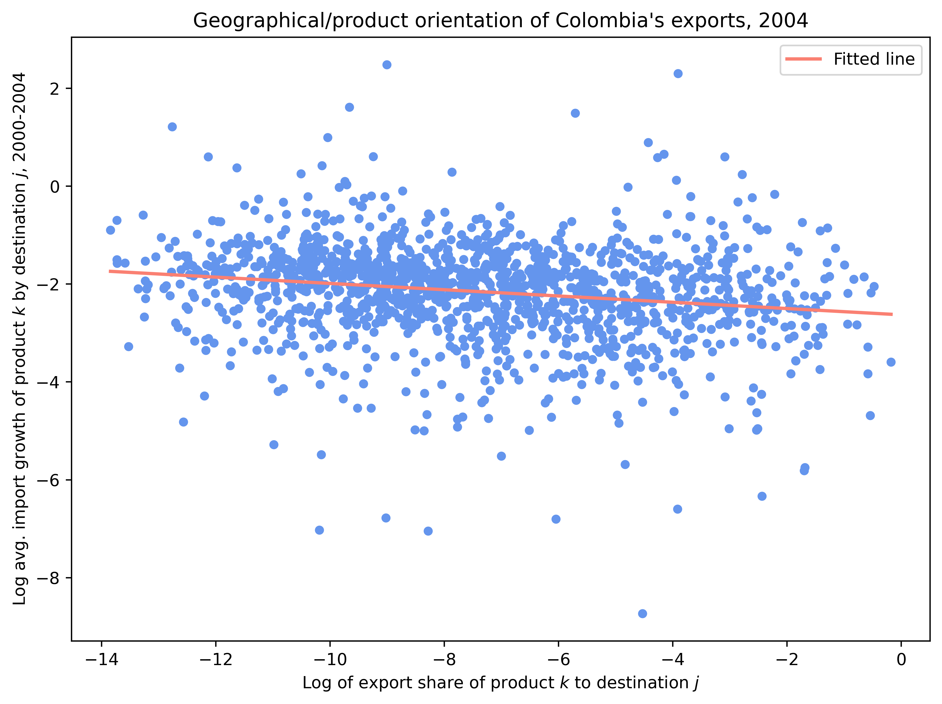
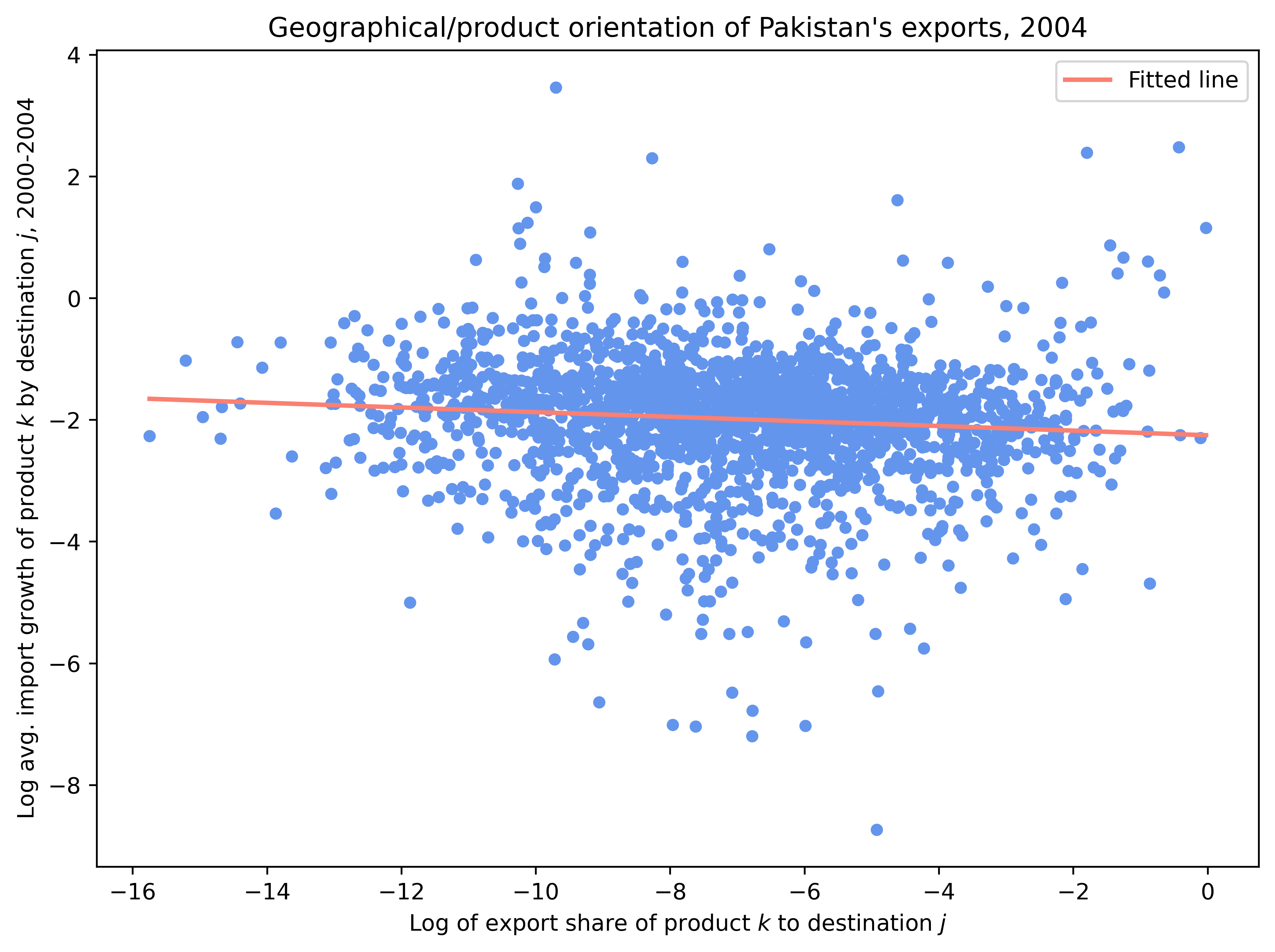
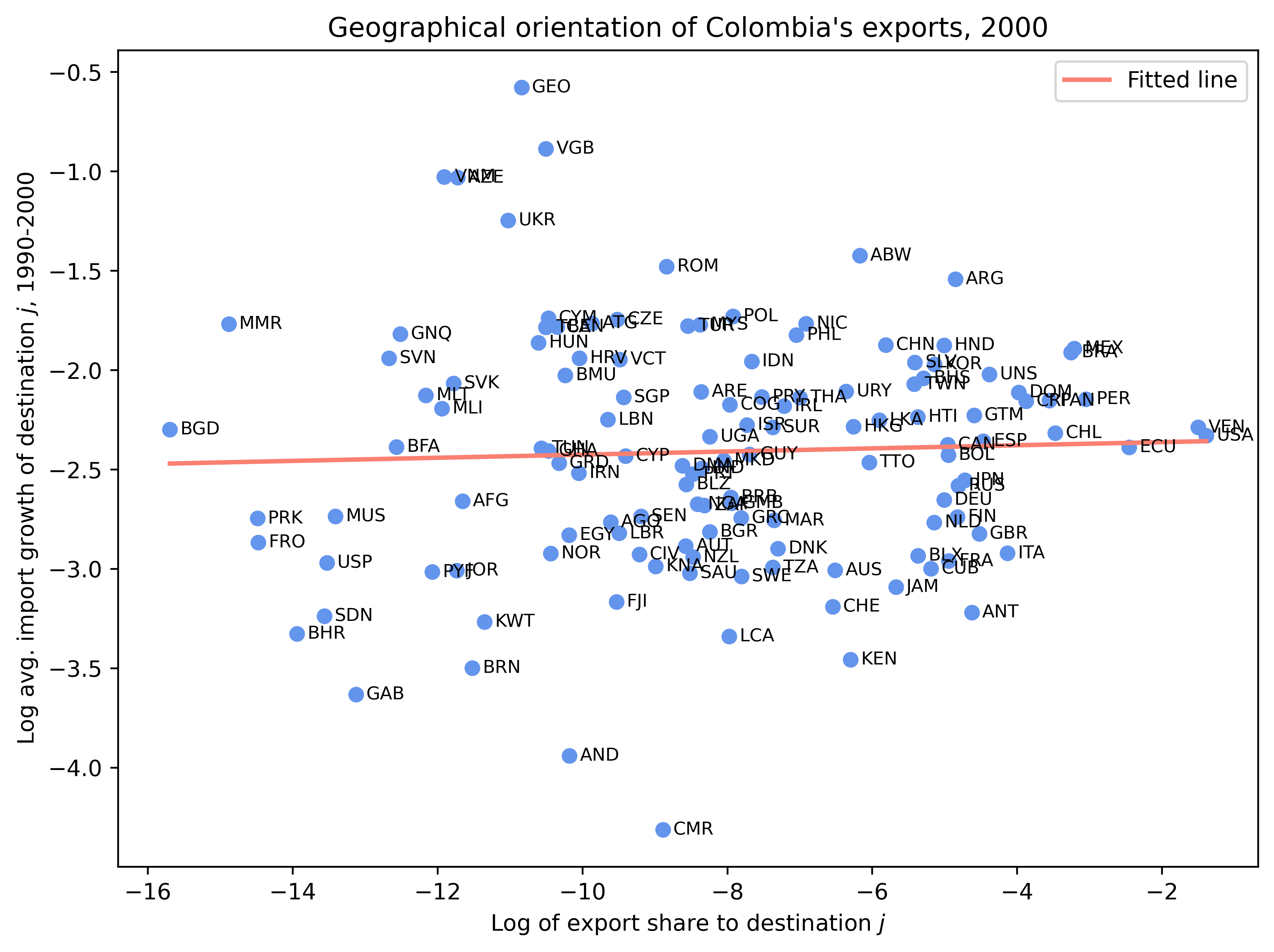
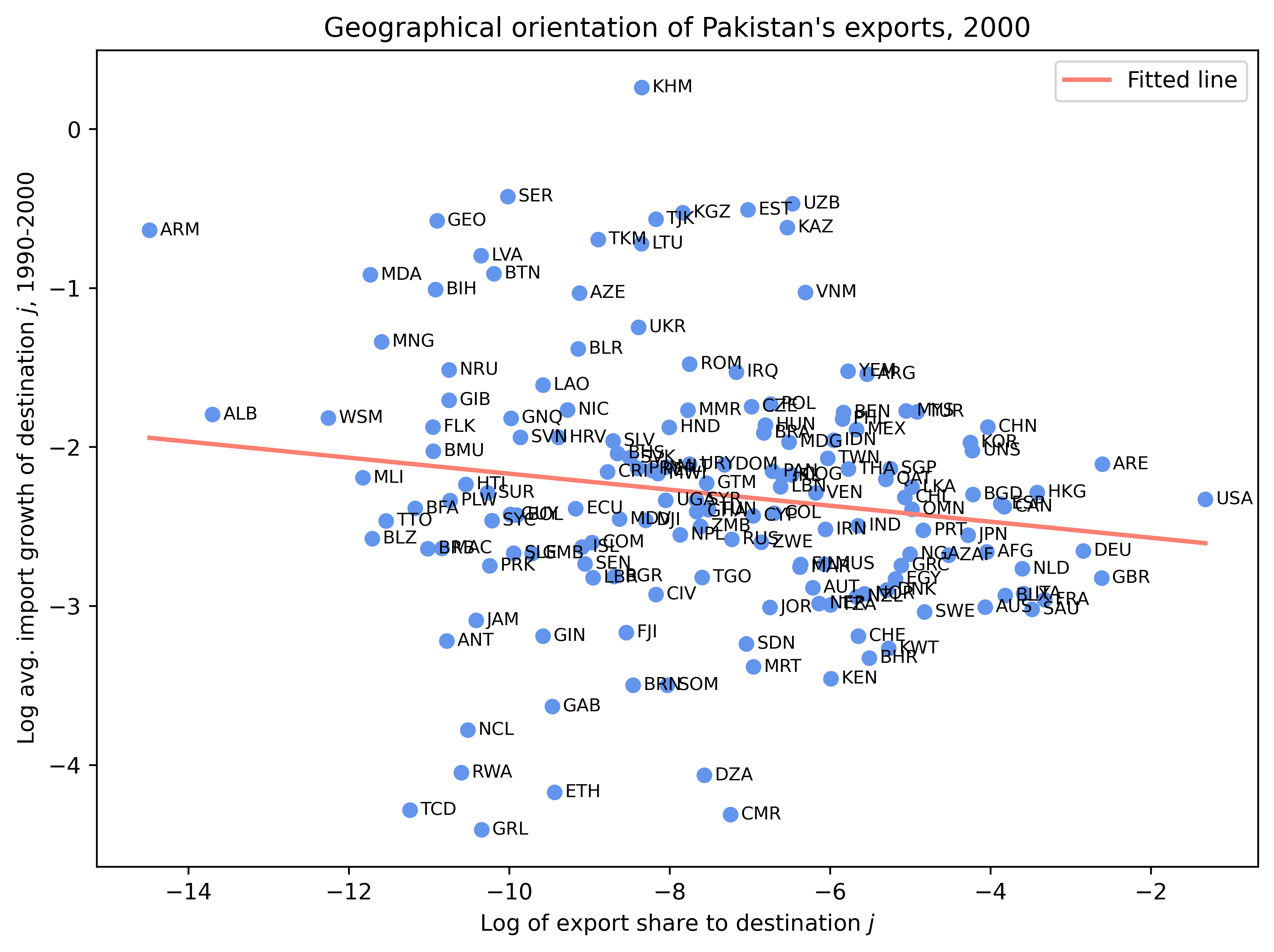
3. 수출 성장의 방향성(1)#
어떤 나라가 수입 성장률이 높은 분야나 나라에 얼마나 많이 수출하는지를 통해, 그 국가의 수출 방향성이 유리한지, 불리한지를 평가할 수 있다.
가령 콜롬비아가 여러 수출 상대국 중, 미국에 압도적으로 수출을 많이 하고 있다고 해보자. 이 상황에서 미국이 아주 빠르게 성장하고, 그래서 미국의 (전세계로부터의) 수입 성장률이 아주 높은 상황이라면 콜롬비아의 수출 방향성이 유리하다고 평가할 수 있다. 간단히 말해서 콜롬비아가 수출 상대국을 잘 선택했다는 의미다.
자국의 전체 수출에서 여러 수출 대상국이 차지하는 비중(로그값)을 \(x\)라고 하고, 지난 10년간 이들 수출 대상국의 평균 수입 성장률을 \(y\)라고 하자. 만약 두 변수 간에 양(음)의 상관관계가 나타난다면, 이는 자국이 상대적으로 성장률이 높은(낮은) 나라에 집중하고 있다는 의미다.
아래 분석은 2000년의 콜롬비아와 파키스탄을 분석한 것이다. 콜롬비아는 수출 방향성이 유리한 반면, 파키스탄은 불리한 것으로 나타난다. 파키스탄의 경우, 성장률이 낮은 걸프 및 중앙아시아 국가들과 인접해 있고, 빠르게 성장하는 인도와의 무역 통합에 실패한 결과로 여겨진다.
데이터(나라별)#
import pandas as pd
import numpy as np
import matplotlib.pyplot as plt

# aBilateralTrade.dta 파일 읽기
df = pd.read_stata("../Data/aBilateralTrade.dta")
df
| ccode | pcode | year | exp_tv | imp_tv | |
|---|---|---|---|---|---|
| 0 | ABW | AIA | 2002 | 773.573975 | 0.000000 |
| 1 | ABW | AIA | 2003 | 63.463001 | 0.000000 |
| 2 | ABW | ALB | 2004 | 0.000000 | 9.815000 |
| 3 | ABW | ANT | 1995 | 475.063997 | 1518.088998 |
| 4 | ABW | ANT | 1996 | 350.091993 | 1608.835018 |
| ... | ... | ... | ... | ... | ... |
| 403130 | ZWE | ZMB | 1999 | 54505.525404 | 16210.871972 |
| 403131 | ZWE | ZMB | 2000 | 69688.172039 | 0.000000 |
| 403132 | ZWE | ZMB | 2001 | 9792.663770 | 12135.245145 |
| 403133 | ZWE | ZMB | 2002 | 175256.748111 | 17891.870960 |
| 403134 | ZWE | ZMB | 2004 | 59845.737700 | 18475.593896 |
403135 rows × 5 columns
수출의 나라별 비중 및 상대국 수입성장률#
# 국가(ccode)와 연도별 총수출액 및 수출 비중 계산
df['tot_exp'] = df.groupby(['ccode', 'year'])['exp_tv'].transform('sum')
df['export_share'] = df['exp_tv'] / df['tot_exp']

# [목적국(pcode)별] 연도별 총수입(여기서는 exp_tv의 합으로 가정) 계산
imp = df.groupby(['pcode', 'year'])['exp_tv'].sum().reset_index().rename(
    columns={'exp_tv': 'totimppcode'})
imp = imp.sort_values(['pcode', 'year'])

# 각 pcode별로 전년도 값과 비교하여 성장률(gamma) 계산
imp['totimppcode_lag'] = imp.groupby('pcode')['totimppcode'].shift(1)
imp['gamma_totimppcode'] = imp['totimppcode'] / imp['totimppcode_lag'] - 1

# 1990~2000년 기간 동안 pcode별 평균 수입 성장률 계산
imp_avg = (imp[(imp['year'] >= 1990) & (imp['year'] <= 2000)]
           .groupby('pcode')['gamma_totimppcode']
           .mean()
           .reset_index()
           .rename(columns={'gamma_totimppcode': 'avg_imp_g_1990_2000'}))

# 원래 데이터와 목적국 수입 성장률 합치기
df = pd.merge(df, imp_avg, on='pcode', how='left')

# 0 이상의 값만 남기고 로그값 생성
df = df[(df['export_share'] > 0) & (df['avg_imp_g_1990_2000'] > 0)]
df['ln_x'] = np.log(df['export_share'])
df['ln_y'] = np.log(df['avg_imp_g_1990_2000'])
# 2000년 자료에서 Colombia("COL")와 Pakistan("PAK") 각각 그래프 생성
for country, title in [
    ("COL", "Geographical orientation of Colombia's exports, 2000"),
    ("PAK", "Geographical orientation of Pakistan's exports, 2000")
]:
    sub = df[(df['ccode'] == country) & (df['year'] == 2000)]
    plt.figure(figsize=(8,6), dpi=500)
    plt.scatter(sub['ln_x'], sub['ln_y'], color='cornflowerblue')

    # 각 점의 바로 오른쪽에 pcode 레이블 표시 (오프셋 적용)
    offset = 0.01 * (sub['ln_x'].max() - sub['ln_x'].min())
    for _, row in sub.iterrows():
        plt.text(row['ln_x'] + offset, row['ln_y'], str(row['pcode']),
                 fontsize=8, va='center')

    # 선형 피팅
    slope, intercept = np.polyfit(sub['ln_x'], sub['ln_y'], 1)
    x_fit = np.linspace(sub['ln_x'].min(), sub['ln_x'].max(), 100)
    plt.plot(x_fit, intercept + slope * x_fit, color='salmon',
             label='Fitted line', linewidth=2)

    plt.xlabel("Log of export share to destination $j$")
    plt.ylabel("Log avg. import growth of destination $j$, 1990-2000")
    plt.title(title)
    plt.legend()
    plt.tight_layout()
    plt.show()
4. 수출 성장의 방향성(2)#
어떤 나라가 수입 성장률이 높은 분야나 나라에 얼마나 많이 수출하는지를 통해, 그 국가의 수출 방향성이 유리한지, 불리한지를 평가할 수 있다.
바로 앞 절에서는 수출하는 상대 나라만을 고려했으나, 수출 제품과 상대 나라를 동시에 고려하면서 수출의 성장 방향성을 평가할 수 있다.
즉, 특정 제품(\(k\))이 특정 대상국(\(j\))으로 수출되는 비중과, 그 제품/대상국의 지난 10년간 평균 수입 성장률을 비교하는 것이다. 만약 두 변수 간에 음의 상관관계가 나타난다면, 이는 자국이 상대적으로 성장률이 낮은 제품에 집중하고 있다는 의미다. 정부가 해당 부문에 투자하여 외연적 증가(extensive margin)를 촉진할 필요가 있음을 의미한다고 볼 수도 있다.
데이터(제품/나라별)#
# UNCTAD (2012) 원래 데이터세트가 용량이 너무 큼
# BilateralTrade.dta 파일 불러오기
BilateralTrade = pd.read_stata("../Data/BilateralTrade.dta")
BilateralTrade = BilateralTrade[BilateralTrade['year'] > 2000]
BilateralTrade.to_csv("../Data/BilateralTrade.csv")
# BilateralTrade.csv 파일 읽기
df = pd.read_csv("../Data/BilateralTrade.csv")
df
| Unnamed: 0 | ccode | pcode | year | isic2_3d | imp_tv | imp_q | imp_uv | exp_tv | exp_q | exp_uv | id | |
|---|---|---|---|---|---|---|---|---|---|---|---|---|
| 0 | 0 | ABW | AIA | 2002 | 311 | 0.000 | NaN | NaN | 773.574 | 433812.0 | 1.783201 | 1.0 |
| 1 | 1 | ABW | AIA | 2003 | 311 | 0.000 | NaN | NaN | 63.463 | 50000.0 | 1.269260 | 1.0 |
| 2 | 2 | ABW | ALB | 2004 | 351 | 8.452 | 11125.0 | NaN | 0.000 | NaN | NaN | 2.0 |
| 3 | 3 | ABW | ALB | 2004 | 352 | 1.363 | 1312.0 | NaN | 0.000 | NaN | NaN | 3.0 |
| 4 | 28 | ABW | ARE | 2003 | 311 | 0.000 | NaN | NaN | 79.050 | 127609.0 | NaN | 10.0 |
| ... | ... | ... | ... | ... | ... | ... | ... | ... | ... | ... | ... | ... |
| 1189499 | 5563250 | ZWE | ZMB | 2002 | 385 | 52.346 | NaN | NaN | 518.514 | NaN | NaN | 545571.0 |
| 1189500 | 5563251 | ZWE | ZMB | 2004 | 385 | 46.147 | 942.0 | 48.988320 | 121.252 | 19096.0 | 6.206012 | 545571.0 |
| 1189501 | 5563265 | ZWE | ZMB | 2001 | 390 | 61.541 | NaN | NaN | 7.266 | NaN | NaN | 545572.0 |
| 1189502 | 5563266 | ZWE | ZMB | 2002 | 390 | 32.965 | NaN | NaN | 720.208 | NaN | NaN | 545572.0 |
| 1189503 | 5563267 | ZWE | ZMB | 2004 | 390 | 51.433 | 18167.0 | 2.831122 | 195.610 | 127486.0 | 1.534365 | 545572.0 |
1189504 rows × 12 columns
수출의 제품/나라별 비중 및 제품/나라의 수입성장률#
# 국가(ccode), 제품(isic2_3d), 연도별 총수출액 및 수출 비중 계산
df['tot_exp'] = df.groupby(['ccode', 'isic2_3d', 'year'])['exp_tv'].transform('sum')
df['export_share'] = df['exp_tv'] / df['tot_exp']

# 목적국(pcode) & 제품(isic2_3d)별 연도별 총수입 계산
imp = (df.groupby(['pcode', 'isic2_3d', 'year'])['exp_tv']
       .sum()
       .reset_index()
       .rename(columns={'exp_tv': 'totimppcode'}))
imp = imp.sort_values(['pcode', 'isic2_3d', 'year'])
imp['totimppcode_lag'] = imp.groupby(['pcode', 'isic2_3d'])['totimppcode'].shift(1)
imp['gamma_totimppcode'] = imp['totimppcode'] / imp['totimppcode_lag'] - 1

# 2000~2004년 동안 (pcode, isic2_3d)별 평균 수입 성장률 계산
imp_avg = (imp[(imp['year'] >= 2000) & (imp['year'] <= 2004)]
            .groupby(['pcode', 'isic2_3d'])['gamma_totimppcode']
            .mean()
            .reset_index()
            .rename(columns={'gamma_totimppcode': 'avg_imp_g_2000_2004'}))

# 원래 데이터와 합치기
df = pd.merge(df, imp_avg, on=['pcode', 'isic2_3d'], how='left')

# 0 이상의 값만 남기고 로그값 생성
df = df[(df['export_share'] > 0) & (df['avg_imp_g_2000_2004'] > 0)]
df['ln_x'] = np.log(df['export_share'])
df['ln_y'] = np.log(df['avg_imp_g_2000_2004'])
df
| Unnamed: 0 | ccode | pcode | year | isic2_3d | imp_tv | imp_q | imp_uv | exp_tv | exp_q | exp_uv | id | tot_exp | export_share | avg_imp_g_2000_2004 | ln_x | ln_y | |
|---|---|---|---|---|---|---|---|---|---|---|---|---|---|---|---|---|---|
| 4 | 28 | ABW | ARE | 2003 | 311 | 0.000 | NaN | NaN | 79.050 | 127609.0 | NaN | 10.0 | 22402.759 | 0.003529 | 0.113866 | -5.646859 | -2.172732 |
| 32 | 66 | ABW | ARG | 2002 | 369 | 71.167 | 347562.0 | 0.204761 | 11.067 | 66.0 | 167.681800 | 27.0 | 249.617 | 0.044336 | 0.185952 | -3.115960 | -1.682266 |
| 39 | 78 | ABW | ARG | 2003 | 381 | 33.982 | 2854.0 | 11.906800 | 0.508 | 30.0 | 16.933330 | 30.0 | 1532.282 | 0.000332 | 0.218641 | -8.011787 | -1.520324 |
| 41 | 81 | ABW | ARG | 2002 | 382 | 0.000 | NaN | NaN | 0.603 | 31.0 | 19.451610 | 31.0 | 1135.912 | 0.000531 | 0.281489 | -7.541029 | -1.267663 |
| 45 | 87 | ABW | ARG | 2003 | 384 | 0.000 | NaN | NaN | 3.352 | 449.0 | 7.465479 | 33.0 | 1794.105 | 0.001868 | 0.475528 | -6.282704 | -0.743329 |
| ... | ... | ... | ... | ... | ... | ... | ... | ... | ... | ... | ... | ... | ... | ... | ... | ... | ... |
| 1189499 | 5563250 | ZWE | ZMB | 2002 | 385 | 52.346 | NaN | NaN | 518.514 | NaN | NaN | 545571.0 | 4747.323 | 0.109222 | 0.113193 | -2.214369 | -2.178662 |
| 1189500 | 5563251 | ZWE | ZMB | 2004 | 385 | 46.147 | 942.0 | 48.988320 | 121.252 | 19096.0 | 6.206012 | 545571.0 | 964.111 | 0.125766 | 0.113193 | -2.073335 | -2.178662 |
| 1189501 | 5563265 | ZWE | ZMB | 2001 | 390 | 61.541 | NaN | NaN | 7.266 | NaN | NaN | 545572.0 | 1158.477 | 0.006272 | 0.064259 | -5.071656 | -2.744836 |
| 1189502 | 5563266 | ZWE | ZMB | 2002 | 390 | 32.965 | NaN | NaN | 720.208 | NaN | NaN | 545572.0 | 56468.068 | 0.012754 | 0.064259 | -4.361891 | -2.744836 |
| 1189503 | 5563267 | ZWE | ZMB | 2004 | 390 | 51.433 | 18167.0 | 2.831122 | 195.610 | 127486.0 | 1.534365 | 545572.0 | 15059.569 | 0.012989 | 0.064259 | -4.343646 | -2.744836 |
755741 rows × 17 columns
for country, title in [
    ("COL", "Geographical/product orientation of Colombia's exports, 2004"),
    ("PAK", "Geographical/product orientation of Pakistan's exports, 2004")
]:
    sub = df[(df['ccode'] == country) & (df['year'] == 2004)]
    plt.figure(figsize=(8,6), dpi=500)

    # 산점도 그리기
    plt.scatter(sub['ln_x'], sub['ln_y'], color='cornflowerblue', s=20)

    # 선형 피팅
    slope, intercept = np.polyfit(sub['ln_x'], sub['ln_y'], 1)
    x_fit = np.linspace(sub['ln_x'].min(), sub['ln_x'].max(), 100)
    plt.plot(x_fit, intercept + slope * x_fit, color='salmon',
             label='Fitted line', linewidth=2)

    plt.xlabel("Log of export share of product $k$ to destination $j$")
    plt.ylabel("Log avg. import growth of product $k$ by destination $j$, 2000-2004")
    plt.title(title)
    plt.legend()
    plt.tight_layout()
    plt.show()